Bayesian Power Analysis at Calm with Google's Causal Impact Library

By George Hayward & Frank Hu

At Calm, we strive to be as data-driven as possible.

That means we run a lot of experiments and quasi-experiments—especially when it comes to important business questions.

One such question is whether Calm should purchase ad space on its own branded keywords.

Ideally, we’d run a classic randomized controlled trial to see how exposure to the ad affects users. But, for privacy reasons, we can’t always track who views a particular ad at a user level or assign individuals into perfect test and control groups.

To address this challenge, we turn to a quasi-experimental approach similar in spirit to difference-in-differences, but implemented via Google’s Causal Impact library (a Bayesian Structural Time Series method). Importantly, rather than using the control group’s raw data directly (as in a strict difference-in-differences), Causal Impact uses the control group to construct a counterfactual function for the treatment group. If we can identify two comparable markets that exhibit parallel trends in a key metric we want to track, we can label one market as control and one as treatment. Then, by measuring “before versus after” differences across both markets, we can reasonably isolate the ad’s impact—despite the lack of a fully randomized assignment.

When it comes to these kinds of time-series analyses, Bayesian regressions are our tool of choice, since samples aren't truly independent. Traditional OLS (“ordinary least squares”) regressions assume samples are independently and identically distributed (i.i.d.), which simply isn’t the case for time-series data that can exhibit autocorrelation, seasonality, and trends. In these types of situations, comparing a result to a prior expectation seems more intuitive.

Designing a Bayesian experiment is often non-trivial, and running a Bayesian power analysis can be tricky. Yet that Bayesian power analysis will guide our decision for how long to run the quasi-experiment, which is a business critical key budgeting decision.

So here, in this post, we wanted to share one approach we used at Calm to complete a rigorous Bayesian power analysis in a difference-in-differences related quasi-experiment designed to answer an age-old question in advertising: should a business purchase ad space on its own branded keywords?

---

Executive Summary

Before we can run the quasi-experiment, we must first design it.

And a key component of the design, and the topic of this blog post is determining how long should we run the quasi-test to confidently detect a meaningful lift?

Because we’re using weekly aggregated data—where each point can be correlated with neighboring points—a standard (frequentist) A/B test may underestimate sample size needs.

Here, we leverage Google’s Causal Impact library (a Bayesian approach) to run multiple simulations (bootstrapping) around a hypothesized effect size. This generates a distribution of p-values (Causal Impact's Bayesian version of a p-value), enabling us to see how many weeks of data we need before we’re likely to reach statistical significance.

Why Do We Care?

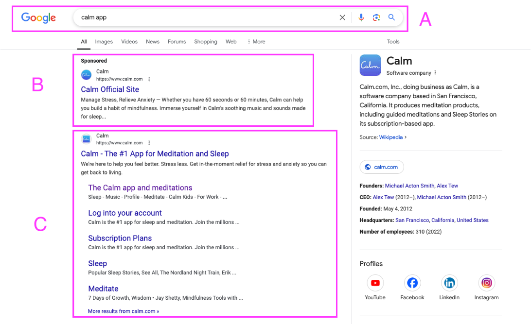
The ultimate business question: If A and C are present, do we also need B?

Calm has a finite advertising budget, and we want to test whether bidding on our own brand keywords is worthwhile. This test diverts resources from our broader marketing plan, so we need an accurate read on:

1. Test Duration: How many weeks of data are required to reliably detect a meaningful lift in brand-based web traffic?
2. Methodology: A time-series experiment with weekly aggregations often violates the independence assumption of standard A/B tests. Further, we've opted to run a difference-in-differences-like quasi-experiment. And we'll want to know how long to run it.

What Is a 'Meaningful' Lift?

When running a power analysis, a few general concepts are true regardless of Bayesian or frequentist design: the bigger the sample size, the greater the power; the longer the test is run, the greater the power.

Before beginning the statistical work, it's important to decide what kind of effect would be enough to make a business decision (i.e. what’s practically significant). At minimum, we want to detect that effect.

What effect is practically significant is dependent on the business context of your test, but, for Calm, in this quasi-experiment, we wanted to detect a 3% difference in a top-of-funnel web traffic metric of our control and treatment. In other words, we'd want to be able to detect a web traffic difference of at least 3%. The idea behind this is that clicks communicate the user’s intention. Perhaps without the ad we would see more organic traffic (clicks) because the ad was cannibalizing traffic that would flow to us regardless. But perhaps without the ad we would see less organic traffic because the ad played a defensive role preventing other ads from scooping away our traffic.

Why Difference-in-Differences Approach?

If we want to study the impact of a given ad's lift on organic web traffic, we need to somehow compare a world where a control group of users see the ad, and a treatment group of users do not see the ad. And, ideally, the only difference between these two independent and random groups would be that one group sees the ad. However, in the world of advertising this is not possible.

Due to privacy concerns, we can't always get a user-level readout of who clicked on an ad. And we similarly can't assign users into a test and control group who may stumble upon a Calm ad.

The next best step would be to find two different markets that are comparable, and make one the control and one the treatment. Assuming that we can achieve this, it still has the problem that they are different groups, there will be many unattributable self-selections into either group, and there can be seasonal impacts that would obscure the real impact of the ad.

If we can confirm that these two markets exhibit parallel trends on our key metric, we can pair them for a quasi-experiment. Note that in a purely frequentist difference-in-differences design, we would directly subtract the control’s outcome from the treatment’s outcome. In this approach, we instead use Google’s Causal Impact BSTS framework to estimate the counterfactual from the control market’s time series, which then gets compared to the treatment market. By applying the treatment (ads) to one market while leaving the other as control, we compare pre- and post-treatment differences to test our null hypothesis—that turning off ads has no effect on trends. This design allows us to estimate the ad's true impact despite the inability to run a randomized controlled experiment.

Why Bayesian?

Traditional frequentist A/B tests assume i.i.d. (independent and identically distributed) samples, which rarely holds for time-series data. Google’s Causal Impact implements a Bayesian structural time-series model, accounting for autocorrelation and trend components in the data. This Bayesian structural time-series model framework is closely related to difference-in-differences ideas but is more flexible in how it constructs the counterfactual from control data, rather than simply subtracting one time series from another. It yields a posterior distribution and tail-area p-value that align more closely with how real-world traffic data behaves over time.

A layperson can understand a p-value as “the odds we’d see this randomly.” Once we have that number, we can use it to make a business decision. Critically, Google’s Causal Impact library makes this number (or perhaps, more specifically, Causal Impact's Bayesian version of a p-value) straightforward to calculate, and with that calculation we can make distributions if we run the library many times.

What’s Interesting About This Technique?

1. Time-Series Awareness: We avoid naive weekly-sample independence assumptions by accounting for autocorrelation and trends. This aligns more closely with how real traffic data behaves and prevents misleading conclusions that arise from treating time-series data as fully independent. By leveraging Google’s Causal Impact library, we effectively perform a differences-in-differences-style analysis but with built-in mechanisms to model real-world traffic fluctuations. This leads to more robust estimates and a more realistic view of how the treatment effect evolves over time, especially crucial when running power analyses to determine how long we need to observe an effect before drawing a conclusion.
2. Bootstrapped Effects: Instead of applying a fixed 3% lift, we randomly sample effect sizes from a normal distribution around 3% (±0.5%). This acknowledges real-world variability and provides a more realistic sense of how the true effect might fluctuate week to week.
3. Why Conventional Power Calculations Don’t Work: In the differences-in-differences quasi-experimental setup—where parallel trends become our best replacement for perfect randomization—standard power formulas for i.i.d. data no longer apply. Time-series dependencies, seasonality, and unobserved confounders can invalidate the typical assumptions behind standard power analyses. By simulating many possible outcomes, i.e., bootstrapping, under these more realistic conditions, we can better estimate how long an experiment needs to run before we can confidently detect our target effect size.
4. Distribution of P-values: By running multiple simulations (e.g., 1,000), we can see how often the resulting p-values fall below 0.05. This gives a direct sense of “power” in the Bayesian context—how likely it is we’ll detect an effect—without making overly simplistic assumptions about data independence.

Methodology Overview

1. Data Source

   • We use historical web traffic data from two states, state_A_redacted (treatment) and state_B_redacted (control), spanning from January 2024 to early 2025.
   • The weekly data is aggregated, and each point could be autocorrelated with prior weeks.

2. Simulation

   • Train a Bayesian regression model with pre-period data (Causal Impact’s underlying structural time-series).
   • Forecast out for X future weeks for each state independently.
   • Intervene: For the treatment state, apply (1 + effect) to the forecasted weeks. The effect is drawn from a normal distribution centered at 3% (±0.5%).
   • Join the modified treatment and unmodified control series to create our “synthetic” post-intervention dataset.

3. Causal Impact & P-value Extraction

   • Run Google’s CausalImpact on the dataset, specifying the pre-period (no effect) and post-period (with effect) dates.
   • Capture the posterior p-value from the output summary.

4. Bootstrapping

   • Repeat the simulation step multiple times (e.g., 1,000).
   • Collect the distribution of p-values.
   • Evaluate how many p-values are below 0.05 for different test durations (4 weeks, 6 weeks, 8 weeks, etc.).

Results and Recommendations

• 4 Weeks: The majority of simulations yield p-values above 0.05, suggesting we lack power.
• 6 Weeks: The median p-value often drops closer to or below 0.05, making it more likely to detect a 3% effect.
• 8 Weeks: Even greater consistency in achieving p-values below 0.05, providing stronger confidence.
• 10 weeks: Top consistency in achieving p-values below 0.05, providing strongest confidence.

In practice, we advise running the test for at least 6 weeks, with 8 weeks being more reliable.

A Limitation To Be Aware Of

One important callout is a limitation inherent to this approach: unlike traditional A/B tests, we can’t run these Bayesian time-series quasi-experiments indefinitely. The core model is a forecast model, and as with any forecast, accuracy tends to degrade the farther out you try to predict. Eventually, there’s a point where each additional week of data adds more noise than signal, which can actually hurt power rather than help it. That’s when extending the test duration becomes less useful, and our attention should shift to our other key lever: the Minimum Detectable Effect. In short, if we can’t gain confidence by waiting longer, we may need to detect larger effects instead.

---

Code Snippets

Below are key Python code snippets. You can copy these directly into your own environment or notebook. File paths and variable names will need adaptation. Finally, we wrote this code bespoke for the way we built our dataframes; your data professionals can adjust some of the function for your company's own proprietary data.

1. Imports & Seed Setup

# When developing, feel free to turn these warnings on.
import warnings
warnings.filterwarnings('ignore')

# These imports are based on Google's Causal Impact Python documentation.
# See -> https://github.com/google/tfp-causalimpact/blob/main/docs/quickstart.ipynb
import tensorflow_probability as tfp
import tensorflow as tf
import random
import matplotlib.pyplot as plt
import pandas as pd
import numpy as np
import causalimpact

tfd = tfp.distributions

# Reproducibility
SEED = 42
np.random.seed(SEED)
tf.random.set_seed(SEED)
random.seed(SEED)

2. Simulation Function

def simulate_intervention_with_forecast(
    df,
    state_treated,         
    state_control,        
    metric,                
    date_column,          
    analysis_start,        
    analysis_end,         
    forecast_steps,        
    begin_intervention_date,  
    effect_duration=None,     
    effect=0.1,              
    effect_type='multiplicative',  
    rename_for_causalimpact=False,
    effect_distribution=None
):
    """
    This function simulates an intervention in a time series forecast, ensuring 
    independent forecasts for the control and treatment states.
    
    - If effect_distribution is provided, each forecast step's effect 
      for the treatment group is drawn from a normal distribution.
    - Otherwise, a constant effect is used.

    In most cases, you'd want to used the effect_distribution, but we have left the   
    constant effect setting in as an option you find useful in certain possible 
    instances. 
    """

    # Convert dates
    analysis_start_dt = pd.to_datetime(analysis_start)
    analysis_end_dt = pd.to_datetime(analysis_end)
    intervention_dt = pd.to_datetime(begin_intervention_date)

    # Filter and pivot data
    df_filtered = df.copy()
    df_filtered[date_column] = pd.to_datetime(df_filtered[date_column])
    df_filtered = df_filtered[
        (df_filtered[date_column] >= analysis_start_dt) & 
        (df_filtered[date_column] <= analysis_end_dt)
    ]
    df_filtered = df_filtered[df_filtered['state'].isin([state_treated, state_control])]

    df_pivot = df_filtered.pivot(
        index=date_column, 
        columns='state', 
        values=metric
    ).astype(float)

    # Mark affected period for historical data
    affected_period = df_pivot.index >= intervention_dt
    if effect_duration:
        affected_period &= (
            df_pivot.index < intervention_dt + pd.Timedelta(weeks=effect_duration)
        )
    
    # Determine constant or distribution-based effect
    if effect_distribution is not None:
        # Single constant effect for the historical portion
        constant_effect = np.random.normal(
            loc=effect_distribution['mean'], 
            scale=effect_distribution['sd']
        )
    else:
        constant_effect = effect

    # Apply effect to the historical portion
    if effect_type == 'multiplicative':
        df_pivot.loc[affected_period, state_treated] *= (1 + constant_effect)
    else:
        df_pivot.loc[affected_period, state_treated] += constant_effect

    # Forecasting future weeks
    last_date = df_pivot.index.max()
    forecast_dates = pd.date_range(
        start=last_date + pd.Timedelta(weeks=1),
        periods=forecast_steps,
        freq='W'
    )

    last_control = df_pivot[state_control].iloc[-1]
    last_treated = df_pivot[state_treated].iloc[-1]

    noise_scale_control = 0.05 * last_control
    noise_scale_treated = 0.05 * last_treated

    control_forecast = (
        np.linspace(last_control, last_control * 1.05, forecast_steps)
        + np.abs(np.random.normal(0, noise_scale_control, size=forecast_steps))
    )

    treated_forecast = (
        np.linspace(last_treated, last_treated * 1.05, forecast_steps)
        + np.abs(np.random.normal(0, noise_scale_treated, size=forecast_steps))
    )

    # Apply effect in the forecast period
    if effect_distribution is not None:
        effects = np.random.normal(
            loc=effect_distribution['mean'],
            scale=effect_distribution['sd'],
            size=forecast_steps
        )
    else:
        effects = np.full(forecast_steps, effect)

    if effect_type == 'multiplicative':
        treated_forecast *= (1 + effects)
    else:
        treated_forecast += effects

    forecast_df = pd.DataFrame(
        {state_control: control_forecast, state_treated: treated_forecast},
        index=forecast_dates
    )

    # Combine historical and forecast data
    combined = pd.concat([df_pivot, forecast_df])

    # Optional renaming for CausalImpact
    if rename_for_causalimpact:
        combined = combined.rename(columns={state_treated: 'y', state_control: 'x1'})

    return combined

3. Single Simulation & Fitting Causal Impact

# Example usage for Calm; this will certainly differ for your company
state_treated = 'state_A_redacted'
state_control = 'state_B_redacted'
metric = 'all_visits'

simulated_data = simulate_intervention_with_forecast(
    df=calm_ua_data,             # your DataFrame
    state_treated=state_treated,
    state_control=state_control,
    metric=metric,
    date_column='event_week',
    analysis_start='2024-01-01',
    analysis_end='2025-04-15',
    forecast_steps=10,
    begin_intervention_date='2025-02-01',
    effect_duration=10,
    effect=0.03,  # Overridden if effect_distribution is provided
    effect_type='multiplicative',
    rename_for_causalimpact=False,
    effect_distribution={'mean': 0.03, 'sd': 0.005}
)

# Define pre and post periods
pre_period = ('2024-01-10', '2025-01-31')
post_period = ('2025-02-01', '2025-04-15')

impact = causalimpact.fit_causalimpact(
    data=simulated_data,
    pre_period=pre_period,
    post_period=post_period
)

# Extract the p-value
p_value = impact.summary['p_value'].iloc[0]
print(f"Single simulation p-value: {p_value:.4f}")

4. Bootstrapping the P-value Distribution

num_simulations = 1000
p_values = []

for _ in range(num_simulations):
    simulated_data = simulate_intervention_with_forecast(
        df=calm_ua_data,
        state_treated=state_treated,
        state_control=state_control,
        metric=metric,
        date_column='event_week',
        analysis_start='2024-01-01',
        analysis_end='2025-04-15',  # or adjust for 6 weeks, 8 weeks, etc.
        forecast_steps=10,
        begin_intervention_date='2025-02-01',
        effect_duration=10,
        effect=0.03,  
        effect_type='multiplicative',
        rename_for_causalimpact=False,
        effect_distribution={'mean': 0.03, 'sd': 0.005}
    )
    
    impact = causalimpact.fit_causalimpact(
        data=simulated_data,
        pre_period=pre_period,
        post_period=post_period
    )

    p_values.append(impact.summary['p_value'].iloc[0])

# Analyze and plot
import matplotlib.pyplot as plt

plt.hist(p_values, bins=30, alpha=0.75)
plt.axvline(np.median(p_values), linestyle='dashed', linewidth=1,
            label=f"Median: {np.median(p_values):.3f}")
plt.axvline(0.05, linestyle='dotted', linewidth=1, label="Threshold: 0.05")
plt.xlabel('P-value')
plt.ylabel('Frequency')
plt.title('Bootstrap Distribution of P-values')
plt.legend()
plt.show()

You can vary analysis_end (thereby changing the number of post-intervention weeks) to simulate tests of different lengths—4 weeks, 6 weeks, 8 weeks, etc.—and compare how often the p-values fall under 0.05.

5. Conclusion

Though Bayesian time-series analysis isn’t brand-new in academic circles, many industry teams have yet to adopt it for power calculations or incremental measurement. Our experience suggests that a bootstrapped Bayesian approach can better handle the realities of time-series data and help you determine how long you need to run a test to detect moderate effects (3% in our case).

For our specific scenario:

• 4 Weeks often yields p-values too high to be confident about detecting a 3% lift.
• 6 weeks makes detection more reliable.
• 8 weeks provides even greater certainty.
• 10 weeks provides the strongest certainty.

By sharing our approach, we hope to fill a gap where traditional A/B tests might fail due to correlated weekly samples. We encourage other teams to leverage similar Bayesian frameworks for more robust, real-world experiment design.